Your ML Model Might Need Better Features, Not a Better Algorithm Feature Engineering Explained: A Beginner's Guide

Imagine you're building a machine learning model to predict whether someone will repay a loan, you give the model a dataset containing the borrower's age, monthly income, employment status, loan amount, and repayment history. You train it.

But what if the model could learn something more useful from the same information?

For example, instead of looking at monthly income and loan amount separately, you could calculate how much of the borrower's monthly income would go toward the loan payment.

That new value might tell the model something neither column communicates as directly on its own.

This is feature engineering.

And it's one of those machine learning concepts that sounds complicated until you start looking at ordinary data differently.

What is feature engineering?

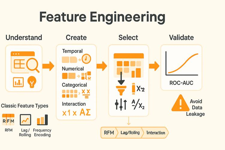
Feature engineering is the process of creating, transforming, or selecting input variables that help a machine learning model learn patterns relevant to a prediction task.

Let's break that down.

Raw data is the information you collect. It might contain numbers, dates, categories, text, missing values, and a few columns that make you wonder why anyone collected them in the first place.

A feature is a piece of information the model uses to make a prediction.

Feature engineering is how we turn the raw information into a representation that is more useful for the model.

For our loan example, raw data might contain:

Raw column	Value
Monthly income	UGX 1,500,000
Monthly loan payment	UGX 450,000
Existing monthly debt payments	UGX 150,000
Employment status	Self-employed
Loan purpose	Business
Previous late payments	2

From these columns, we could derive a feature called debt-to-income ratio:

Formula: DTI Ratio = Monthly Debt Payments / Monthly Income

Calculation: DTI Ratio = 600,000 / 1,500,000 = 0.4 (40%)

That is a debt-to-income ratio of 40%.

The ratio gives the model a compact representation of how much of the borrower's monthly income is already committed to debt payments.

It doesn't guarantee a better prediction, and it isn't a complete measure of creditworthiness. But it gives us a meaningful candidate feature to test.

That's the key idea is that we're not collecting more information. We're making better use of the information we already have.

Why does feature engineering matter?

A machine learning algorithm learns patterns from the representation of data it receives.

If that representation hides a useful relationship, the model may struggle to learn it.

Suppose two borrowers have these profiles:

Borrower	Monthly income	Monthly loan payment
A	UGX 500,000	UGX 200,000
B	UGX 2,000,000	UGX 200,000

Both have the same monthly loan payment.

But the payment represents 40% of Borrower A's income and only 10% of Borrower B's income.

Looking at the loan payment alone doesn't communicate that difference. Combining the information into a ratio makes it easier to represent.

This is one reason a carefully designed feature set can matter as much as, or sometimes more than, switching to a more complicated algorithm.

Of course, the best features depend on the model, the dataset, the prediction task, and how the features are evaluated. Feature engineering is not a guarantee of better performance.

1. Numerical features

Numerical features represent quantities that can be measured or counted.

In a loan repayment dataset, examples include:

• Monthly income

• Loan amount

• Monthly repayment amount

• Number of previous late payments

• Length of employment in months

• Existing monthly debt

Some numerical features are continuous, meaning they can take many values within a range. Income and loan amounts are examples.

Others are discrete counts, such as the number of previous late payments.

Creating useful numerical features

You can combine existing numerical columns to create new ones.

For example:

• Debt-to-income ratio

• Loan amount divided by annual income

• Monthly disposable income

• Number of late payments per year, if the relevant time period is available

• Difference between income and estimated monthly expenses

Here's a simple example:

import pandas as pd

df = pd.DataFrame({
    "monthly_income": [1_500_000, 800_000, 2_000_000],
    "monthly_debt_payments": [600_000, 200_000, 500_000],
    "loan_amount": [5_000_000, 2_000_000, 8_000_000],
})

df["debt_to_income_ratio"] = (
    df["monthly_debt_payments"] / df["monthly_income"]
)

print(df[["debt_to_income_ratio"]])

The new column represents the proportion of monthly income already committed to debt payments.

In a real dataset, we'd also check for zero or missing income values before dividing. We would need to define the time period consistently, too. Comparing monthly debt payments with annual income without converting the units would produce a misleading feature.

One more thing: a ratio is not automatically better than its original columns. Keep it if evaluation shows that it helps, or if it provides another clear benefit.

2. Categorical features

Not all useful information comes as numbers.

A loan application might include:

• Employment status: employed, self-employed, unemployed

• Loan purpose: education, business, housing

• Residence type: rented, owned, family home

• Application channel: branch, mobile app, agent

These are categorical features. They represent groups or labels rather than numerical quantities.

Most traditional machine learning algorithms need categorical values to be represented in a suitable numerical format.

Simply changing labels to numbers can be dangerous.

For example:

Employed      → 1
Self-employed → 2
Unemployed    → 3

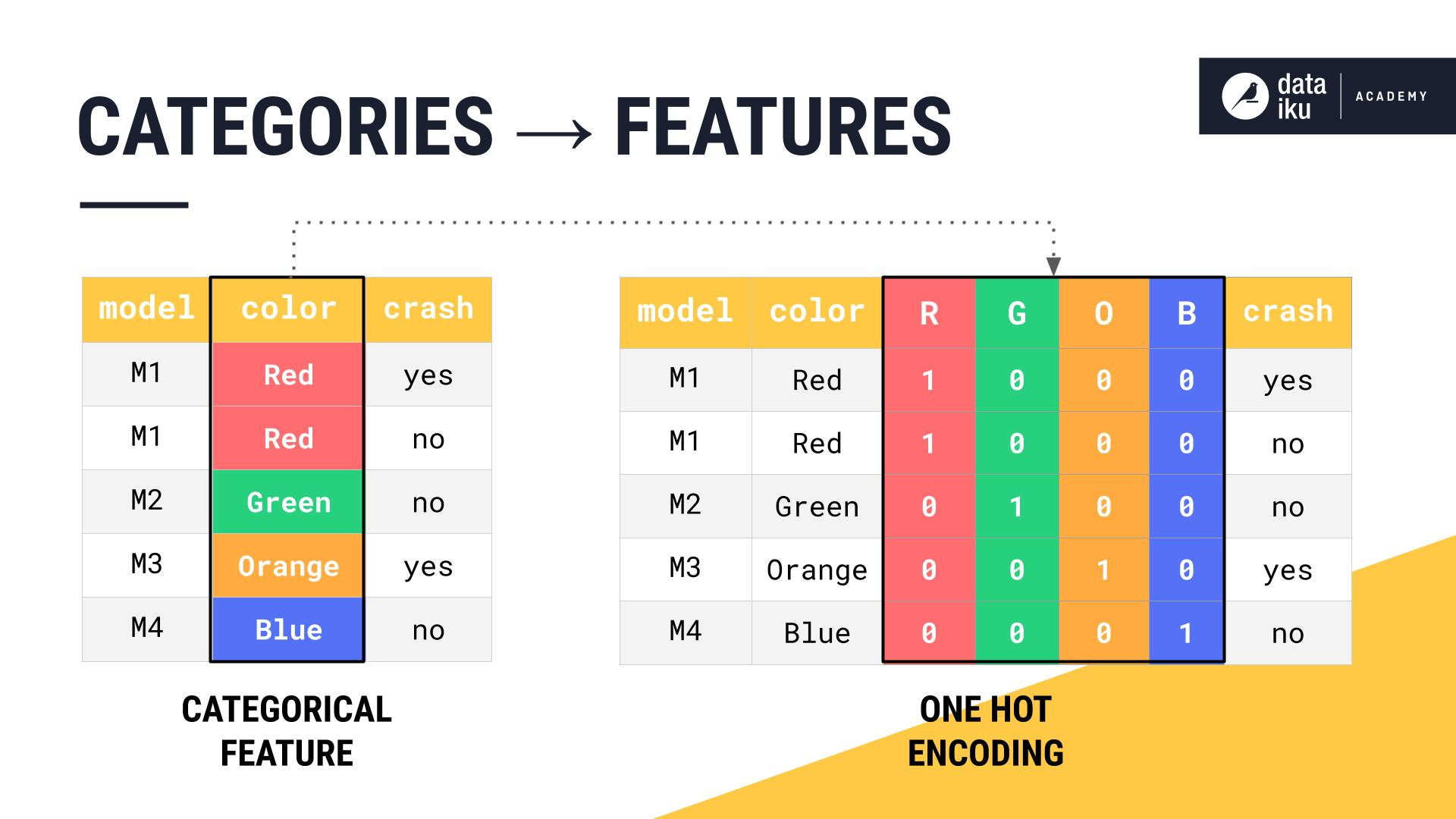
This encoding introduces an apparent order: 3 is greater than 2, which is greater than 1. But employment categories don't necessarily have that numerical relationship. For nominal categories, one common solution is one-hot encoding.

For example:

Employment status	employed	self_employed	unemployed
Employed	1	0	0
Self-employed	0	1	0
Unemployed	0	0	1

Each category gets its own binary feature. In pandas, you can create this representation with:

encoded = pd.get_dummies(
    df,
    columns=["employment_status"],
    dtype=int
)

This assumes your DataFrame contains an employment_status column.

For a production model, be careful about categories that appear during prediction but were not present during training. A fitted encoder in a consistent preprocessing pipeline can handle this more reliably than manually encoding columns each time.

Also, some categories have a genuine order. For example, an explicitly defined education level may be ordinal. Whether to use ordinal encoding depends on the meaning of the categories and the model.

3. Time features

Dates can contain more useful information than their raw values suggest, suppose a borrower has a repayment date of 2026-10-15. A model might benefit from features such as:

• Day of the week

• Month

• Time since the loan was issued

• Number of days since the last repayment

• Number of missed payments within a defined past period

We can extract some calendar features with pandas:

df = pd.DataFrame({
    "application_date": [
        "2026-01-12",
        "2026-06-21",
        "2026-10-05",
    ]
})

df["application_date"] = pd.to_datetime(
    df["application_date"]
)

df["application_month"] = (
    df["application_date"].dt.month
)

df["application_day_of_week"] = (
    df["application_date"].dt.dayofweek
)

print(df)

The dayofweek values range from 0 for Monday to 6 for Sunday.

Whether these features help depends on the problem. A day-of-week feature might be useful for predicting transaction activity, for example, but irrelevant for a particular loan repayment task.

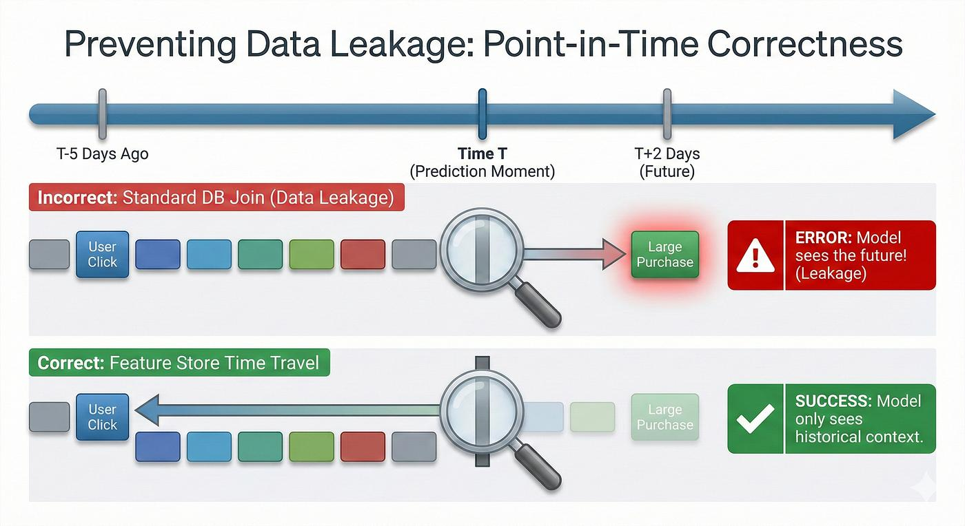
There is also a major warning with time-based data which is to use only information that would have been available at the moment the prediction was made.

If you're predicting repayment at the time a loan application is submitted, you cannot use the borrower's eventual repayment date or future missed payments as input features.

That would be data leakage. We'll get to that shortly.

4. Text features

Loan applications may also contain text, for example, an applicant might write a short explanation of why they need a loan.

Text can contain useful information, but a traditional ML model cannot automatically understand a raw sentence in the same way a human reader does. One simple approach is to convert text into numerical representations.

A common beginner-friendly technique is bag-of-words: represent documents using counts or weights associated with the words they contain. For example, these two phrases contain different terms:

"Buy equipment for my business"

"Pay school fees for my children"

A bag-of-words representation can turn the text into a vector of numerical values indicating which terms occur and how frequently. In Python, scikit-learn's CountVectorizer can do this:

from sklearn.feature_extraction.text import CountVectorizer

texts = [
    "buy equipment for my business",
    "pay school fees for my children",
    "expand my small business",
]

vectorizer = CountVectorizer()

text_features = vectorizer.fit_transform(texts)

print(vectorizer.get_feature_names_out())
print(text_features.toarray())

The vectorizer builds a vocabulary and represents each text using counts from that vocabulary.

This is only one option. TF-IDF can reduce the relative weight of terms that occur frequently across documents, while more advanced NLP systems can use learned embeddings.

For a loan model, though, we should not assume that an applicant's wording reliably predicts repayment. Text features can encode irrelevant patterns or sensitive proxies, and any such use needs careful evaluation for fairness, privacy, and regulatory compliance.

5. Feature scaling

Imagine one feature measures age in years and another measures annual income in Uganda shillings, their numerical ranges are very different. Age might range from 18 to 70, while annual income might range from hundreds of thousands to tens of millions.

Some algorithms are sensitive to these differences in scale. Models based on distances, gradient optimization, or regularization often benefit from appropriate scaling. Two common techniques are standardization and min-max scaling:

Standardization

Standardization transforms a feature using its mean and standard deviation:

z = (x - mean) / standard_deviation

Definitions:

• x: The original value.

• mean: The average calculated from the training data.

• standard_deviation: The standard deviation calculated from the training data.

The transformed values are centered around zero and scaled by the standard deviation, assuming it is nonzero.

Min-max scaling

Min-max scaling maps values to a chosen range, commonly 0 to 1:

x_scaled = (x - x_min) / (x_max - x_min)

Where:

• x_scaled: The new normalized value (typically between 0 and 1).

• x: The original value.

• x_min: The minimum value in the training data.

• x_max: The maximum value in the training data.

This formula assumes the feature has a nonzero range.

Do all models need feature scaling?

No.

Linear models, support vector machines, k-nearest neighbors, and many gradient-based methods can benefit from scaling, depending on the setup.

Tree-based models such as decision trees and random forests generally don't require standardization because their splits depend on feature thresholds rather than distances between raw values.

Scaling also doesn't automatically make a feature more informative. It changes its numerical representation.

One important rule: fit the scaler on the training data, then use that fitted scaler to transform validation, test, and production data. Don't calculate the scaling statistics using the entire dataset before splitting it. That can leak information from evaluation data into the training process.

Scikit-learn pipelines help keep these steps consistent. Its documentation explains both the benefits of preprocessing pipelines and the risks of data leakage. Scikit-learn: Common pitfalls and recommended practices.

6. Feature selection

After creating and preparing features, you might end up with dozens or hundreds of columns.

Do you need all of them?

Not necessarily.

Feature selection is the process of choosing a useful subset of features for a model.

Why might you remove features?

• Some contain very little useful information.

• Some duplicate information already represented elsewhere.

• Some add noise.

• Some make the system more expensive or complicated.

• Some create privacy, fairness, or data-availability concerns.

• Some are only available after the prediction should already have been made.

There are several approaches to feature selection.

Filter methods

These evaluate features using statistical criteria, such as correlation or tests of association. They're relatively simple, but a feature that appears weak on its own might still be useful in combination with other features.

Wrapper methods

These evaluate subsets of features by repeatedly training and assessing a model. They can be computationally expensive because they may require many model fits.

Embedded methods

Some models perform feature selection as part of training. Regularization methods, for example, can shrink certain coefficients toward zero.

Tree-based models also provide feature-importance measures, although those measures must be interpreted carefully. Importance does not prove causation, and correlated features can complicate interpretation.

The goal isn't to keep the smallest possible dataset. It's to find a useful representation that performs well on unseen data and makes sense for the application.

Feature selection must also be performed without using the held-out test set to make decisions. Otherwise, the test set gradually becomes part of the model-development process.

7. Data leakage: the feature engineering mistake to avoid

This is one of the most important parts of the whole topic. Data leakage happens when information that wouldn't legitimately be available at prediction time influences model training or evaluation. The result can be a model that looks excellent during testing but performs much worse when deployed.

Let's return to loan repayment.

Suppose we're predicting whether a borrower will repay a loan when they apply. Our dataset contains:

Feature	Available at application time?
Monthly income	Yes, if collected and verified
Employment status	Yes, if collected
Requested loan amount	Yes
Previous repayment history	Potentially, if historical records are available
Number of missed payments on the new loan	No, not at application time
Final repayment status	No, this is the outcome we're trying to predict

If we use the number of missed payments on the new loan to predict whether the borrower will repay it, we're allowing future information into the model.

The model isn't learning to predict the future, it's getting clues from what happened afterward and that is a serious problem.

How to avoid leakage

First, define the exact moment when the prediction will be made.

Then ask of every feature: would this information genuinely be available at that moment?

Next, split the dataset into training and evaluation sets before fitting preprocessing steps that learn statistics or select features. Fit those steps on the training data only.

For time-dependent tasks, use a time-aware evaluation strategy when appropriate. Randomly splitting historical records can create an unrealistic evaluation if it lets future information influence the past.

Finally, build the feature transformations into a repeatable pipeline so training and prediction use the same rules.

A useful question to keep asking is:

"Would I actually know this value when the model needs to make its prediction?"

If the answer is no, don't use it as an input feature for that prediction.

8. Let's build a small feature engineering example

Let's put some of these ideas together.

We'll create a tiny illustrative loan dataset and engineer a few features using pandas. The dataset is synthetic, it isn't real borrower data, and the example is for learning rather than making actual lending decisions.

import pandas as pd

df = pd.DataFrame({
    "monthly_income": [1_500_000, 800_000, 2_000_000, 1_200_000],
    "monthly_debt_payments": [600_000, 200_000, 500_000, 300_000],
    "loan_amount": [5_000_000, 2_000_000, 8_000_000, 3_000_000],
    "loan_term_months": [12, 10, 24, 12],
    "employment_status": [
        "employed",
        "self-employed",
        "employed",
        "self-employed",
    ],
    "application_date": [
        "2026-01-12",
        "2026-03-18",
        "2026-06-21",
        "2026-10-05",
    ],
    "repaid": [1, 1, 0, 1],
})

# Create a feature from existing numerical columns.
df["debt_to_income_ratio"] = (
    df["monthly_debt_payments"] / df["monthly_income"]
)

# Extract a calendar feature from the application date.
df["application_month"] = (
    pd.to_datetime(df["application_date"]).dt.month
)

# Convert the categorical feature into indicator columns.
df = pd.get_dummies(
    df,
    columns=["employment_status"],
    dtype=int,
)

print(df.head())

Let's walk through what happened.

First, we created debt_to_income_ratio from two existing numerical features.

Second, we extracted the application month from the date. This would be available at application time, assuming the date is recorded correctly.

Third, we encoded employment status into numerical indicator columns.

The repaid column is our target: the outcome the model will learn to predict. It must not be included among the input features.

Also, this small example intentionally leaves out several steps you'd need for a real training pipeline, including splitting the data, handling missing values, validating feature ranges, and checking whether the features are useful.

One final detail: the loan amount and loan term might be used to derive an estimated monthly payment, but only if the repayment schedule and interest assumptions are known. It's better to define the calculation carefully than create a feature that looks meaningful but doesn't represent the actual loan.

9. Putting it into a real ML workflow

Feature engineering doesn't end when you create a few columns in a notebook.

If you're building a model that will be used in production, you need to ensure the same feature logic is applied consistently to training data and new applications.

For example, if your model was trained using a debt-to-income ratio calculated from monthly values, production inference must calculate that ratio using the same definitions and units.

A pipeline can help organize preprocessing and model training. In scikit-learn, you can combine transformations and an estimator so that the same fitted preprocessing steps are applied when making predictions.

This is especially useful for:

• Handling missing numerical values.

• Encoding categorical variables.

• Scaling features where appropriate.

• Selecting features.

• Avoiding inconsistent transformations between training and serving.

For a more complex dataset with numerical and categorical columns, scikit-learn's ColumnTransformer can apply different transformations to different groups of columns, while a Pipeline chains those transformations together with a model.

The broader lesson is that feature engineering is part of the model system, not a one-time notebook trick.

If the feature definitions change, you may need to retrain the model and evaluate the new version. If upstream data changes unexpectedly, feature validation and monitoring can help catch the problem before it silently affects predictions.

What I'm taking away

Feature engineering is about asking better questions of your data, Instead of looking at monthly income and loan amount as unrelated columns, I can ask whether their relationship tells me something useful.

Instead of feeding a model raw dates, I can consider whether the month or elapsed time is relevant.

Instead of assuming every column deserves a place in the dataset, I can question whether it's useful, available at prediction time, and appropriate for the task.

And I need to remember that more features don't automatically mean a better model.

The next time you open a dataset, don't rush straight to choosing an algorithm.

Look at the columns first.

Ask what each one represents, what it leaves out, what useful information you could derive from it, and whether that information would genuinely be available when the prediction is made.

Sometimes the most useful improvement to an ML model starts before the model is trained.

I'm documenting what I'm learning about machine learning and production systems here on Godfident Data. Next, I'll continue exploring the decisions that turn a working model into a reliable system.